Sergey Khashin, List of RK methods

List of some Runge-Kutta methods family

Back to main page
Last update: 2025-07-27

Here you can find some families of Runge-Kutta (RK) methods in Maple (text) file.
For example, classical RK-methods of order 4 is represented by next procedure:

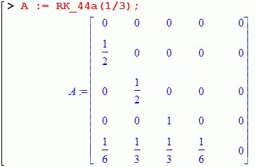
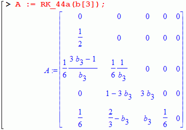
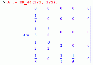
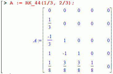
RK_44 := proc(c2, c3)::Matrix;
    local a,d;
	if c2=1/2 then ERROR(`RK_44: c2=1/2`); end if;
	if c2=c3  then ERROR(`RK_44: c2=c3`);  end if;
	if c2=1   then ERROR(`RK_44: c2=1`);   end if;
	if c3=1   then ERROR(`RK_44: c3=1`);   end if;
	d := factor(3-4*(c2+c3)+6*c2*c3);
	if d=0 then ERROR(`RK_set44: 3-4*(c2+c3)+6*c2*c3=0`); end if;
    a := Matrix(5,5);
    a[2,1] := c2;
    a[3,2] := c3*(c3-c2)/(2*c2*(1-2*c2));
    a[3,1] := c3-a[3,2];
    a[4,2] := (c2-1)*(2-c2-5*c3+4*c3*c3)/(2*c2*(c3-c2)*d); 
    a[4,3] := (1-2*c2)*(c3-1)*(c2-1)/(c3*(c3-c2)*d); 
    a[4,1] := 1 - a[4,3] - a[4,2];
    a[5,2] := (1-2*c3)/(12*c2*(c2-1)*(c3-c2)); 
    a[5,3] := (2*c2-1)/(12*c3*(c3-1)*(c3-c2)); 
    a[5,4] := (3-4*c2-4*c3+6*c2*c3)/(12*(c2-1)*(c3-1));
    a[5,1] := 1 - a[5,4] - a[5,3] - a[5,2];
    simplify(a);
end proc;

Maple-file	Feature
rk_methods.txt	Most of the methods are here,
ex_rk_56a.txt	17 examles of rk_56a methods with b2!=0 and small coefficients.
ex_rk_67.txt	Examles of rk_67 methods with small coefficients.
rk_79.txt	Maple-script with 9 stage Runge-Kutta methods of order 7,
rk_79e.txt	RK_79e(c2, c4, c5, c7, c8), with b2=b3=0,
rk_8.txt	11 stage RK methods of order 8.

List of methods:

Name p s Reference Feature

Order 4

RK_44(c2,c3) 4 4 [B1] Classical

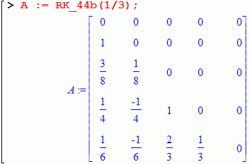
RK_44a(b3) 4 4 [B1] c₂=c₃=1/2

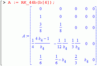
RK_44b(b4) 4 4 [B1] c₂=1, c₃=1/2

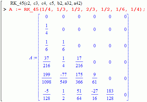
RK_45(c2, c3, c4, c5, b2, a32, a42) 4 5 ? dim = 7

Order 5

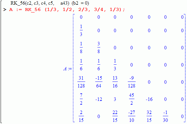
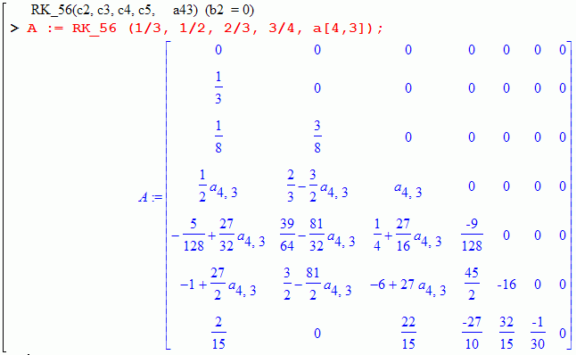
RK_56 (c2, c3, c4, c5, a43) 5 6 [B1] Butcher, b₂=0

RK_56a(c2, c3, c4, c5, b2, a43) 5 6 ? dim=6

Rational poins on RK_56a

RK_56b(c2, c3, c4, a43, e5) 5 6 ? dim=5, b2!=0, c5=c3, c6=1

Order 6

RK_67(c2, c3, c5, c6) 6 7 [B1] Butcher, b₂=0

RK_67a(c3, c5, c6) 6 7 ? b₂<>0, b₁=b₇=1/12

RK_67b(c2, a32, b3) 6 7 ? b₂<>0, c₂=c₃=c₆

Order 7

RK_79(c4, c5) 7 9 [B1] Butcher, b₂=b₃=0

RK_79e(c2,c4,c5,c7,c8) 7 9 - S.Khashin, b₂=b₃=0, five parametes

RK_79d(c2,c3,c4,c5,a52,c7,ind) 7 9 - S.Khashin, b₂=0, b₃≠0

Order 8

RK_8_11(a105, b8) 8 11 [Seka] Assui Kouassi Richard, Seka Hippolyte

RK_8_11(c5,c6,c7,c9,c10) 8 11 - S.Khashin, b₂=b₃=b₄=0,

Name	p	s	Reference	Feature
Order 4
RK_44(c2,c3)	4	4	[B1]	Classical
RK_44a(b3)	4	4	[B1]	c₂=c₃=1/2
RK_44b(b4)	4	4	[B1]	c₂=1, c₃=1/2
RK_45(c2, c3, c4, c5, b2, a32, a42)	4	5	?	dim = 7
Order 5
RK_56 (c2, c3, c4, c5, a43)	5	6	[B1]	Butcher, b₂=0
RK_56a(c2, c3, c4, c5, b2, a43)	5	6	?	dim=6
Rational poins on RK_56a
RK_56b(c2, c3, c4, a43, e5)	5	6	?	dim=5, b2!=0, c5=c3, c6=1
Order 6
RK_67(c2, c3, c5, c6)	6	7	[B1]	Butcher, b₂=0
RK_67a(c3, c5, c6)	6	7	?	b₂<>0, b₁=b₇=1/12
RK_67b(c2, a32, b3)	6	7	?	b₂<>0, c₂=c₃=c₆
Order 7
RK_79(c4, c5)	7	9	[B1]	Butcher, b₂=b₃=0
RK_79e(c2,c4,c5,c7,c8)	7	9	-	S.Khashin, b₂=b₃=0, five parametes
RK_79d(c2,c3,c4,c5,a52,c7,ind)	7	9	-	S.Khashin, b₂=0, b₃≠0
Order 8
RK_8_11(a105, b8)	8	11	[Seka]	Assui Kouassi Richard, Seka Hippolyte
RK_8_11(c5,c6,c7,c9,c10)	8	11	-	S.Khashin, b₂=b₃=b₄=0,

[B1] Butcher, J. C., "Numerical Methods for Ordinary Differential Equations" Second Edition, J. Wiley, Chichester, (2008)
[HNV] Hairer E., Norsett S.P., Wanner G., "Solving ordinary differential equations 1. Nonstif Problems.", 528 p.,Sprigner-Verlag., Berlin Heidelberg (2008)
[Seka] Seka Hippolyte & Assui Kouassi Richard, 2019. "A New Eighth Order Runge-Kutta Family Method," Journal of Mathematics Research, Canadian Center of Science and Education, vol. 11(2), pages 190-199, April.

Methods of order 4

RK_44(c2,c3)

RK_44(c2,c3) - standart 4-stage RK method of order 4.
Restrictions: c2!=1/2, c3!=1, c3!=1, c3!=c2, 3-4(c2+c3)+6 c2 c3 !=0

RK_44a(b3)

In the above function, the condition c2!=c3 must be fulfilled. But in some important cases, it is not performed. Therefore, we provide a separate function that allows you to find such methods.

The matrix created by this function satisfies the conditions:
c2=1/2, c3=1/2, c4=1.
Restrictions: b3!=0

RK_44b(b4)

Another relation must be fulfilled in the RK_44 function: c2!=1.
However, there are RK methods that do not satisfy this condition. There is another function for this case.
c2=1, c3=1/2, c4=1.
Restrictions: b4!=0

Remark. There are no additional methods for which 3-4(c2+c3)+6 c2 c3=0.

RK_45(c2, c3, c4, c5, b2, a32, a42)

Although 5-stage methods of the order 4 are unlikely to be in high demand, for completeness, we present a function that finds such methods.

Methods of order 5

Let the matrix A represent a 6-stage Runge-Kutta method of the 5th order. The coefficients of the matrix must satisfy 17 equations (order conditions) corresponding to trees of weight <=4 [B1, HNV]. First of all, we present a function that implements the well-known 6-stage methods of the order of 5 [B1, HNV].

RK_56 (c2, c3, c4, c5, a43)

Main feature: b2=0

RK_56a(c2, c3, c4, c5, b2, a43)

Now we builds a family of methods for which b2!=0 (in the general case), that is, additional simplifying assumptions are not fulfilled. The dimension of this family is 6 and the methods found by J.Butcher are its special cases for b2=0.

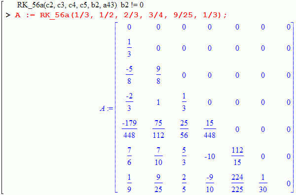
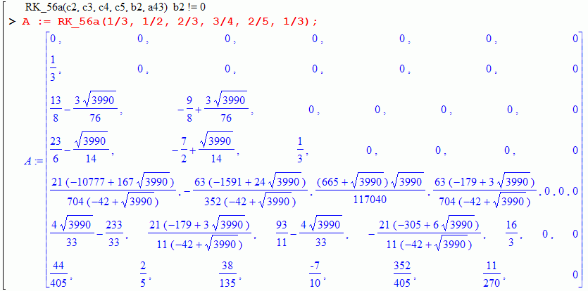
In general, the coefficients of the matrix will contain quadratic irrationalities:

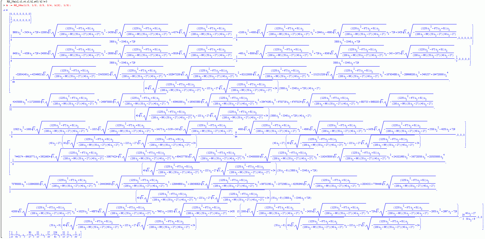
Be carefull! After

we obtain

Rational points

Methods obtained using the function RK_56a will usually return a matrix with irrational numbers.
However, for some values of parameters, the matrix will contain only rational numbers and the coefficients have relatively small denominators.
Here are some such examples.

RK_56a(c2, c3, c4, c5, b2, a43); RK_56a(2/5, 4/5, 3/5, 1/2, 25/24, 3/5); RK_56a(2/5, 1/2, 1/4, 3/4, -125/84, 3/16); RK_56a(1/3, 1/2, 3/4, 4/5, 27/80, 3/4); RK_56a(1/5, 4/5, 3/5, 1/2, 25/96, 3/4); RK_56a(1/5, 4/5, 1/2, 3/5, 25/96, 3/4); RK_56a(2/5, 4/5, 3/5, 1/5, 5/8, 3/5); RK_56a(3/5, 4/5, 2/5, 1/5, -5/18, 13/30); RK_56a(1/5, 4/5, 3/5, 1/2, 25/96, 3/2); RK_56a(1/5, 3/5, 4/5, 1/2, 25/96, 3/2); RK_56a(2/5, 1/2, 3/4, 1/4, -125/84, 3/16); RK_56a(4/5, 2/5, 1/3, 3/5, 25/168, 1/2); RK_56a(3/5, 2/5, 4/5, 1/5, -5/18, 1/30); RK_56a(3/5, 4/5, 2/5, 1/2, 25/72, 13/30); Example:

And Butcher matrices in a text file

RK_56b(c2, c3, c4, a43, e5)

The matrices obtained by the function RK_56a(c2,c3,c4,c5,b2,a43) satisfy the condition c3!=c5 and c6!=1. However, there are methods that do not meet such requirements. They can be obtained using the function RK_56b(c2, c3, c4, a43, e5).

Exapmple:

Methods of order 6

Let the matrix A represent a 7-stage Runge-Kutta method of the 6th order. The coefficients of the matrix must satisfy 37 equations (order conditions) corresponding to trees of weight <=5 [B1, HNV]. First of all, we present a function that implements the well-known 7-stage methods of the order of 6 [B1, HNV].

RK_67(c2, c3, c5, c6)

(b2=0).

RK_67a(c3, c5, c6)

The methods presented above satisfy two simplifying assumptions. Their characteristic feature is the equality b2=0.

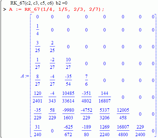
But there is another family of methods. It does not satisfy the second simplifying assumption.

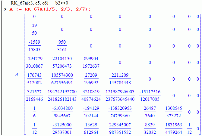
Their characteristic features: b1=b7=1/12 and b2!=0.

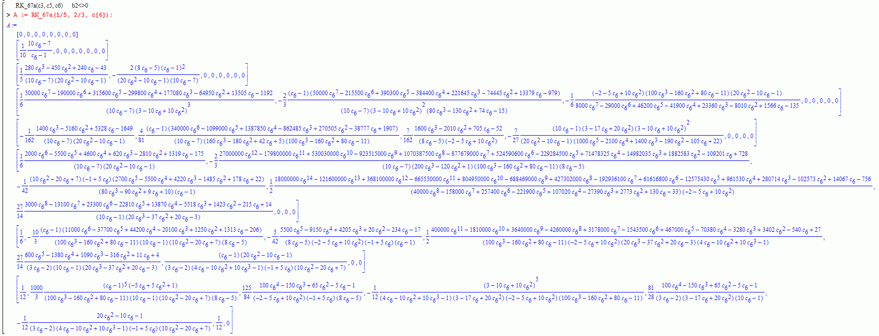
They can be constructed using the function RK_67a(c3, c5, c6).

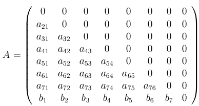
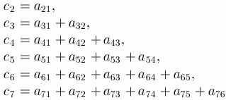
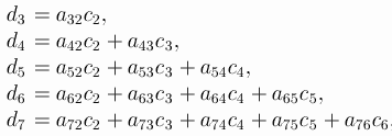
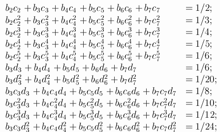
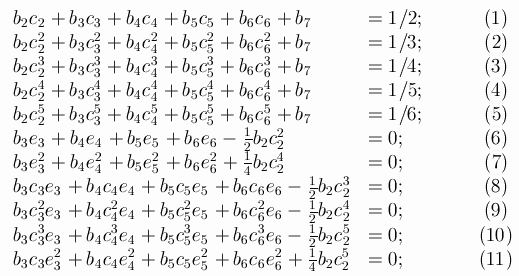
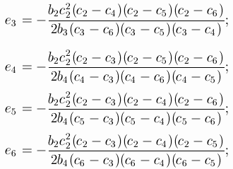
Let A be the extended matrix of the 7-stage RK-method of order 6, A is a lowertrianle matrix of size 8*8 with zero diagonal:

As usual, lets introduce variables c_i:

Lets introduce variables d₃, ..., d₇ by formulas:

In our case c₇=1, d₇=1/2.
Some of order conditions contains only b_i, c_i, d_i:

for k,l > = 0, k+2l < p, or

Lets introduce variables e₃, ..., e₇ by formulas: e_i=d_i-c_i²/2:

(e₇=0). So:

One can express variables e₃,e₄,e₅,e₆ from equations (6,8,9,10):

and

where

Then

where

and

is elementary symmetric functions of variables x₁, x₂, x₃.
With the substitution of found solutions in the complete system of orders conditions, it turns out that not every set of the above the free variables (c₂,c₃,c₄,c₅,c₆), there is a solution of the full system. More exactly:

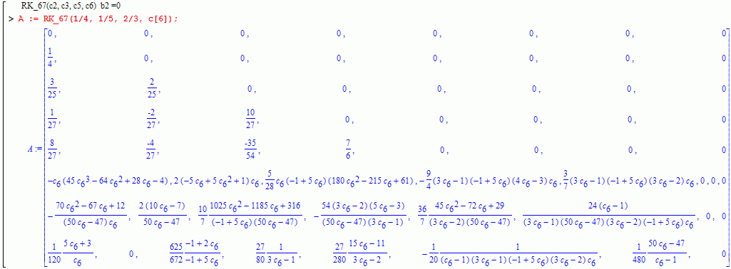
You can even leave one of the parameters undefined:

RK_67b(c2, a32, b3)

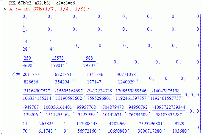
In addition to the two families of methods mentioned above, it is possible to build another one.

Their characteristic features: c2=c3=c6,
c4 = c2/(15*c2^2 - 10*c2 + 2);
c5 = (9*c2-4)/(3*(5*c2-2));

They can be constructed using the function RK_67b(c3, c5, c6).

Example:

You can even leave one of the parameters undefined:

Methods of order 7

RK_79(c4, c5)

In J.Butcher's book (see reference above), page 178, a two-dimensional family of methods of order 7 is constructed.

These methods can be built using the function RK_79(c4, c5).

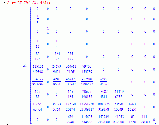
You may also use:

or even:
,
but be careful!

RK_79e(c2,c4,c5,c7,c8)

In separate Maple-text-file rk_79e.txt, function RK_79e.

5-dimensional family of 9-step RK methods of order 7.

If parameters c2,c4,c5,c7,c8 are rational, then all matrix coefficients will also be rational.

Example:

,

,

with free c2:
,

You can take other pameters free, but be ready for a long formulas and a large amount of memory.

For example, command

>A := RK_79e(c2, c4, 4/7, c7, c8):

need 204M of memory! And

> length(A);

17756

RK_79d(c2,c3,c4,c5,a52,c7,ind)

In separate Maple-text-file rk_79.txt, function RK_79d.

6-dimensional family of 9-step RK methods of order 7.

All parameters must be rational.

Arguments c2,c3,c4,c5,a52,c7 are obvious.

When finding the matrix, you have to solve the quadratic equation. We need to choose one of its two roots:
ind = 1: 1st root
ind = 2: 2nd root

All the coefficients of the result matrix are quadratic irrationalities.

Example:
,

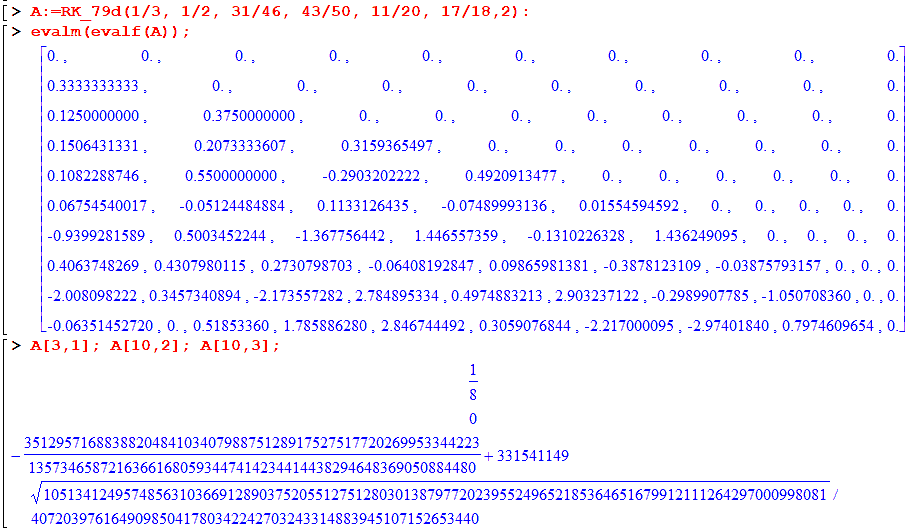Usually, all the coefficients of the result matrix are quadratic irrationalities. But it is possible to find a matrix with rational coefficients.


> read `\\w\\RUNGE_KU\\MAPLE\\rk_79.txt`:
> c3:=1/3: c4:=2/3: c5:=3/4: a52:=1:  
# Rational points on elliptic curve:
> eq17 := RK79_c7c8(c3,c4,c5,a52);
> P2:=ratPoints(eq17,10):
> for k from 1 to nops(P2) do
>   print(k, ` P2~=`, evalf(P2[k]), ` len=`, length(P2[k]), ` eq17=`, eq17(P2[k][1], P2[k][2]) );
> end do:
> c7 := P2[1][1]; c8 := P2[1][2];
> A  := RK_79a(c3,c4,c5,a52,c7,c8);
> evalf(A);

The point is that eq17 is a bi-quadratic function:

,
So the equation eq17=0 gives an elliptic curve in variables (c7,c8).
The function ratPoints (from rk_79.txt) using the group law find 10 rational points on this curve.
Unfortunately, the values are rising fast:


     [ 1836169365208  590253357997083915732956147028 ]
P1 = [ -------------, -------------------------------]
     [14375031772353  1006076034939621277811626968047]
 

     [191413646630639454100269817605058328881625109  590253357997083915732956147028 ]
P2 = [---------------------------------------------, -------------------------------]
     [158225722728039129214784412615341412861584569  1006076034939621277811626968047]

 ...

However, all the coefficients of the matrix are rational.

Methods of order 8

RK_8_11s(a105,b8)

This method was developed by Seka Hippolyte & Assui Kouassi Richard [Seka]
For b8 = 49/180 and a105 = 1/9, the Cooper-Verner obtained.

We will not consider these methods in more detail, since they are a special case of the following, more general function.

RK_8_11(c5,c6,c7,c9,c10)

In separate Maple-text-file rk_8.txt, we have a function RK_8_11.
It's main feature is b2=b3=b4=0.

res_8.txt - the last two matrices in the text file.

But be carefull! Random selection of parameters may not be very convinient!

Main page